하나둘셋넷

house price 예측하기

라이브러리 불러오기

import pandas as pd

데이터 읽기

df = pd.read_csv('kc_houseprice.csv')
display(df.columns)
df.head()

df.info()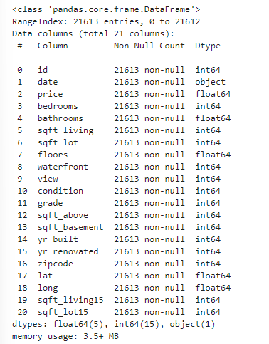

# 현재 date의 데이터만 object 타입임을 확인할 수 있다.

데이터 전처리

# 위에서 date 열을 보면 20141209T~~~~ 형식으로 되어있어서 활용하기 어렵다.

# 따라서 분석에 유효한 앞에 4글자만 가져오도록 한다.

# 이후에는 float 타입으로 변환

버릴 데이터를 찾아보자

df['date'] = df.loc[:,'date'].str[:4]
df['date'] = df.loc['date'].astype(float)
display(df.info())
display(df)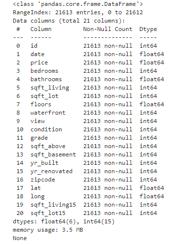

타겟 데이터 분리

target = 'price'
x = df.drop(['sqft_living15', 'sqft_lot15' ,target], axis = 1)
y = df[target]

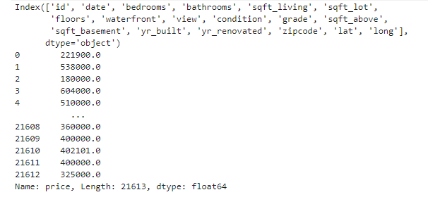
display(x)
display(x.columns)
display(y)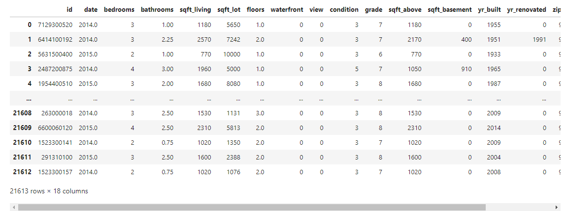

훈련용 데이터 분리하기

from sklearn.model_selection import train_test_split

x_train, x_test, y_train, y_test = train_test_split(x, y, test_size = 0.2, random_state = 2023)

데이터 스케일링

from sklearn.preprocessing import MinMaxScaler
scaler = MinMaxScaler()
x_train = scaler.fit_transform(x_train)
x_val = scaler.transform(x_val)

모델 설계

nfeatures = x_train.shape[1]

from keras.backend import clear_session
clear_session()

from keras.layers import Dense, Dropout
from keras.models import Sequential

model_DNN = Sequential()
model_DNN.add(Dense(18, input_shape = (nfeatures, ), activation = 'relu') )
model_DNN.add(Dropout(0.3) )
model_DNN.add(Dense(4, activation = 'relu'))
model_DNN.add(Dense(1) )

model_DNN.summary()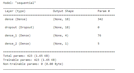

Param # 

출력 노드 * ( 입력노드 + 1 ) = Param

18 * ( 입력차원 + 1 ) = 18 * 19 = 342

4 * ( 입력차원 + 1 ) = 4 * 19 = 76

1 * ( 입력차원 + 1 ) = 1 * 5 = 5

따라서, 342 + 76 + 5 = 423

Total params : 423과 일치한다.

모델 컴파일 및 학습

from keras.optimizers import Adam

model_DNN.compile(optimizer = Adam(learning_rate = 0.01), loss = 'mse')
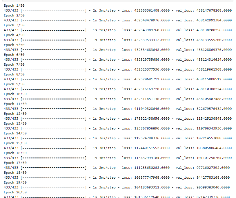
hist = model_DNN.fit(x_train, y_train, epochs = 50, validation_split = 0.2).history

검증

from sklearn.metrics import *

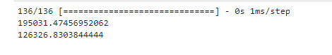
pred = model_DNN.predict(x_val)

print(mean_squared_error(y_val, pred, squared = False) ) # RMSE
print(mean_absolute_error(y_val, pred)

K-means

• yellowbrick
• 선행 작업 문자형 수치형으로
• 선행 작업  scaling

#[문제 1] 필요 라이브러리 로딩
# numpy, pandas, matplotlib, seaborn, os 를 임포트 하기

import pandas as pd
import numpy as np
import matplotlib.pyplot as plt
import seaborn as sns
import os

# 시각화 표에서 에러나는 부분 글꼴 셋팅

plt.rc("font", family = "Malgun Gothic")
sns.set(font="Malgun Gothic", 
rc={"axes.unicode_minus":False}, style='white')

# 지수표현(소수점 2자리까지 나타내기)

pd.options.display.float_format = '{:.2f}'.format


# [문제 2] 스케일링 한 데이터 불러오기
# 1. data 변수에 'scaler_data.csv' 파일을 불러와서 할당, 인코딩은 utf-8
# 2. data 변수 호출해서 상위 5개 확인해보기

data = pd.read_csv('scaler_data.csv', encoding = 'UTF -8 ')


import yellowbrick

from sklearn.cluster import KMeans
from yellowbrick.cluster import KElbowVisualizer

# Elbow Method 활용해서 k 값 구하기

• yellowbrick의 k-Elbow Mehod를 활용해서 최적의 k 값을 구하기(k값 결정하기 쉽게 도와주는 함수)

#Elbow Method를 통해 최적의 군집 수 도출을 해보자.

from yellowbrick.cluster import KElbowVisualizer
from sklearn.cluster import KMeans

# 1. 모델 선언하기 (random_state=2023, n_init=10 으로 설정)
model_E = KMeans(random_state=2023, n_init=10)

# 2. KElbowVisualizer 에 k-means 모델과 k값 넣어서 만들기(Elbow_M 에 할당)
# k값은 k=(3,11)사이의 값중에서 찾는 것으로 넣으면 된다.

Elbow_M = KElbowVisualizer(model_E, k=(3, 11))

# 3. Elbow 모델 학습하기(fit)

Elbow_M.fit(data)

# 4. Elbow 모델 확인하기(show()활용)

Elbow_M.show()

선행 작업 문자형 수치형으로

# 상품타입'범주를 인코딩 해보기
# loc를 활용해서 '기본,중급'을 0으로 변환/ '고급'을 1로 변환

data_choice.loc[(data_choice['상품타입']=='기본') | (data_choice['상품타입']=='중급'),'상품타입'] = 0
#---------------------------------------------------------------
data_choice.loc[data_choice['상품타입']=='고급','상품타입'] = 1


# 데이터 안의 정보는 수치형이지만 dtype은 아직 object 이다. 범주형을 수치형으로 변경해 주자!
# astype-> float64 활용해서 변경 후 확인
data_choice_n = data_choice_n.astype('float64')

선행 작업 scaling

# min-max-scaler & standard-scaler import!(sklearn의 processing 활용)
from sklearn.preprocessing import MinMaxScaler, StandardScaler

#. scaler라는 변수에 MinMaxScaler 넣어주기
scaler = MinMaxScaler()

#. 'data_choice_n'을 'scaler_data' 변수에 fit-transform으로 fit 하기!
# 각 열을 스케일링
scaler_data = scaler.fit_transform(data_choice_n)
print("scaler_data",scaler_data)

# 컬럼은 이전 dataframe('data_choice_n') 에서 그대로 가져와서 'scaler_data.columns'에 할당하기
# 컬럼 가져오기
scaler_columns = data_choice_n.columns

pd.DataFrame(scaler_data, columns = data_choice_n.columns)



# 스케일링이 잘 되었는지 'scaler_data' 데이터를 확인해보자
scaler_data = pd.DataFrame(scaler_data, columns = data_choice_n.columns)
scaler_data

회귀 KNeighborsRegression

라이브러리 불러오기

import pandas as pd
import matplotlib.pyplot as plt
from sklearn.model_selection import train_test_split

변수 제거", "데이터 분리", "가변수화

# 변수 제거
del_cols = ['컬럼명']
data.drop(del_cols, axis=1, inplace = True)

# 데이터 분리
target = '타겟 컬럼'
x = data.drop(target, axis=1)
y = data.loc[:,target]

# 가변수화
dum_cols = ['컬럼명', '컬럼명', '컬럼명']
x = pd.get_dummies(x, columns = cols, drop_first = True)

학습용 평가용 데이터 분리, 정규화

# 학습용, 평가용 데이터 분리
from sklearn.model_selection import train_test_split
x_train, x_test, y_train, y_test = train_test_split(x, y, test_size = 0.3, random_state = 1)

# 정규화
from sklearn.preprocessing import MinMaxScaler

scaler = MinMaxScaler()
scaler.fit(x_train)
x_train = scaler.transform(x_train)
x_test = scaler.transform(x_test)

성능 예측

from sklearn.neighbors import KNeighborsRegression

분류 - LogisticRegression

1. 라이브러리 불러오기

import pandas as 

impot numpy as np

import maplotlib.pyplot as plt

import seaborn as sns

2. 데이터 불러오기

data = pd.read_csv('데이터.csv')

3. 학습용 평가용 데이터

from sklearn.model_selectoin import train_test_split

x_train, x_test, y_train, y_test = train_test_split(x, y, test_size = 0.3, random_state=2023)

4. 모델링

# 1단계 : 불러오기

from sklearn.linear_model import LogisticRegression

from sklearn.metrics import confision_matrix, classification_report

# 2단계: 선언하기

model = LogisticRegression()

# 3단계 : 학습하기

model.fit(x_train, y_train)

# 4단계 : 예측하기

y_pred = model.predict(x_test)

# 5단계 평가하기

print(confusion_maxtrix(y_test, y_pred))

print(classification_report(y_test, y_pred))

필기

필기 2

XGBClassifier

• XGBClassifier에 대한 GPT의 답변
• params 대입 방법

XGBClassifier에 대한 GPT의 답변

params 대입 방법

# 라이브러리 불러오기

import numpy as np
import  pandas as pd
import matplotlib.pyplot as plt

from sklearn.model_selection import train_test_split

# 데이터 불러오기

data = pd.read_csv(path)

# target 확인
target = 'ADMIT'

# 데이터 분리
x = data.drop(target, axis=1)
y = data[target]

# 7:3으로 분리
x_train, x_test, y_train, y_test = train_test_split(x, y, test_size=0.3, random_state=1)

# 선언하기
model = XGBClassifier(max_depth=5, random_state=1)

# 학습하기
model.fit(x_train,y_train)

# 예측하기

y_pred = model.predict(x_test)

# 평가하기

print(confusion_matrix(y_test, y_pred))
print(classification_report(y_test,y_pred))

내용

• model 저장하기 joblib

내용

• PCA
• PCA 코드
• 주성분 누적 분산 그래프 elbow method

주성분 누적 분산 그래프 - 그래프를 보고 적절한 주성분의 개수를 지정(elbow method) - x축 : PC 수 - y축 : 전체 분산크기 - 누적분산크기
	# 코드 plt.plot( range(1, n+1), pca.explained_variance_ratio_, marker = '.') plt.xlabel('No. of PC')

군집분석

시각화

# 코드 plt.scatter(result['x1'], result['x2'], c=result['predicted'], alpha =0.5) plt.scatter(centers['x1'], centers['x2'], s = 50, marker ='D', c='r'

적정한 k 값 찾기

	# k means 모델을 생성하게 되면 inertia 값을 확인 가능 model.inertia_
from sklearn.cluster import KMeans kvalues = range(1, 10) inertia = [] for k in kvalues:     model = KMeans(n_clusters = k, n_init = 'auto')     model.fit(x)     inertias.append(model.inertia_) # 그래프 그리기 plt.plot(kvalues, inertias, '-o') plt.xlabel('numbers of clusters, k') plt.ylabel('inertia')

# 적정한 k 값을 찾은 경우

분석 방법

지도 학습 분류 문제

랜덤 포레스트 분류

1. 환경 준비
2. 데이터 준비
3. 모델링

지도 학습 분류 문제

결정나무 분류

1. 환경 준비
2. 데이터 이해
3. 데이터 준비
4. 모델링
5. 기타

• graphviz
• 변수 중요도