회귀 KNeighborsRegression
라이브러리 불러오기
import pandas as pd
import matplotlib.pyplot as plt
from sklearn.model_selection import train_test_split
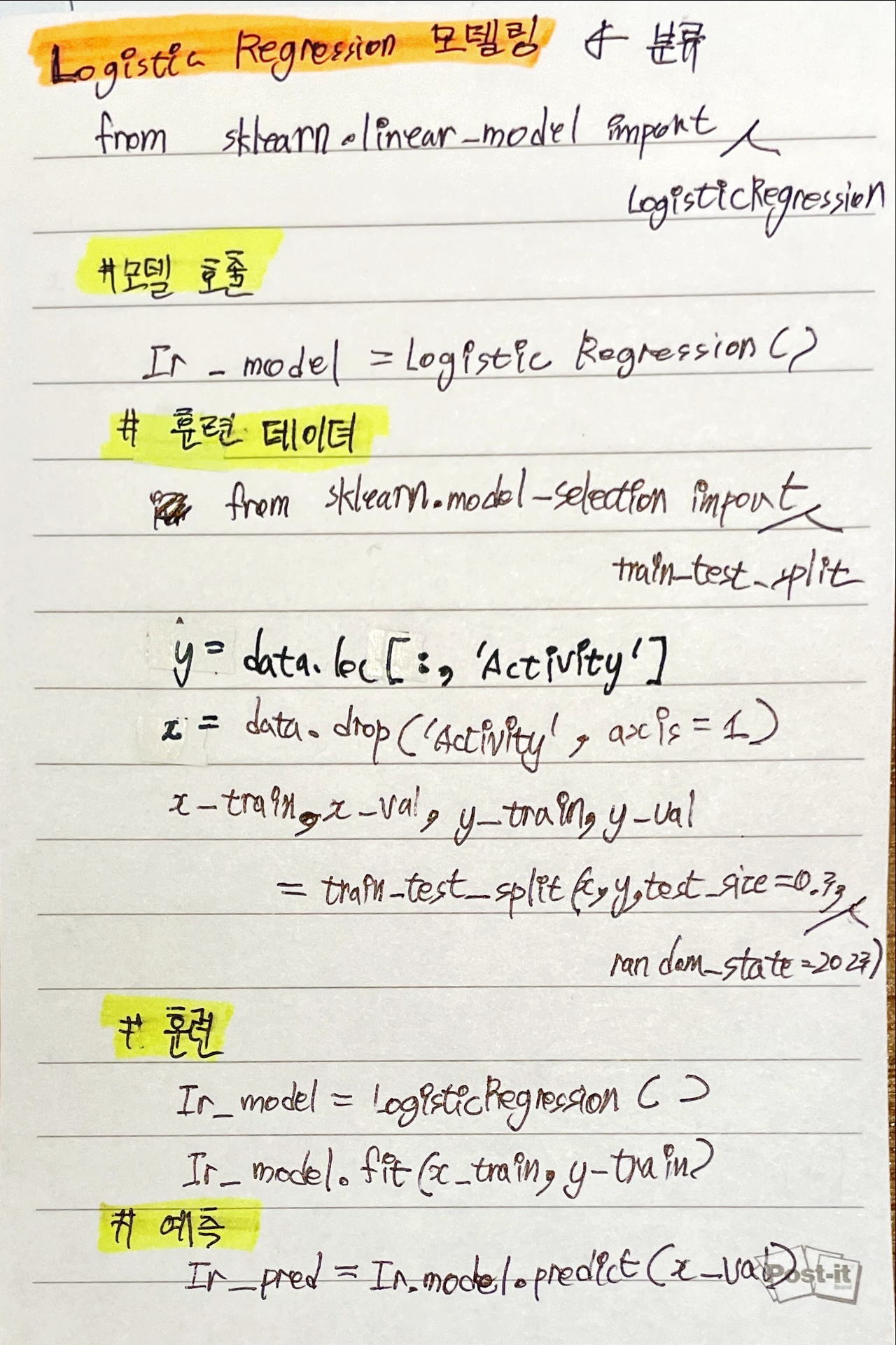
변수 제거", "데이터 분리", "가변수화
# 변수 제거
del_cols = ['컬럼명']
data.drop(del_cols, axis=1, inplace = True)
# 데이터 분리
target = '타겟 컬럼'
x = data.drop(target, axis=1)
y = data.loc[:,target]
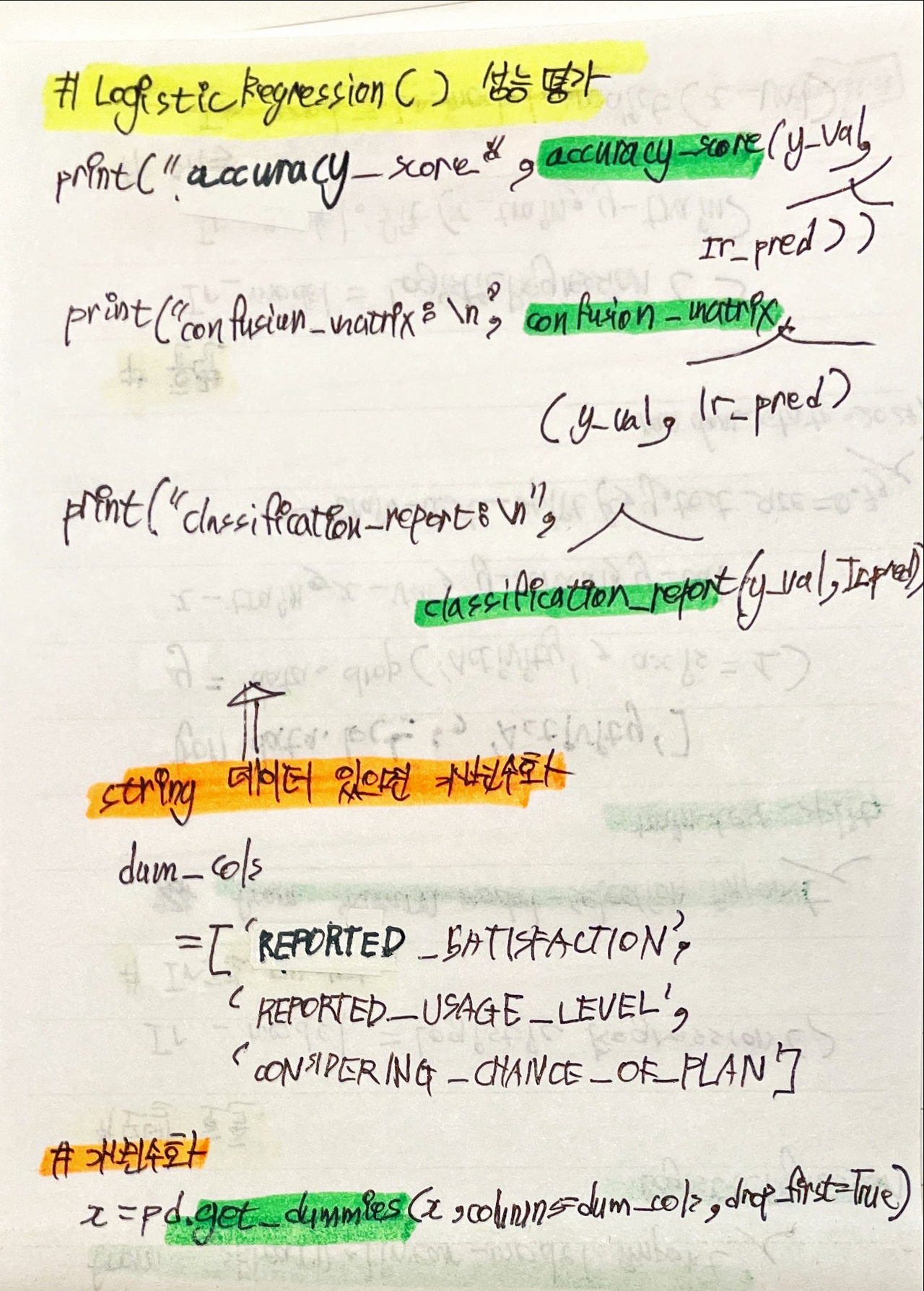
# 가변수화
dum_cols = ['컬럼명', '컬럼명', '컬럼명']
x = pd.get_dummies(x, columns = cols, drop_first = True)
학습용 평가용 데이터 분리, 정규화
# 학습용, 평가용 데이터 분리
from sklearn.model_selection import train_test_split
x_train, x_test, y_train, y_test = train_test_split(x, y, test_size = 0.3, random_state = 1)

# 정규화
from sklearn.preprocessing import MinMaxScaler

scaler = MinMaxScaler()
scaler.fit(x_train)
x_train = scaler.transform(x_train)
x_test = scaler.transform(x_test)
성능 예측
from sklearn.neighbors import KNeighborsRegression